
Smart Chess Board
12-778: Sensors, Circuits and Data Interpretation/Management for Infrastructure Systems (Fall 2022)
Instructor : Prof. Mario Bergés , Professor of Civil and Environmental Engineering, CMU
Table of Contents
Acknowledgements
The project would not be successful without the support of Brian Belowich, CEE Facilities & Lab Engineer. Throughout the project, Brian has always been supportive and encouraging with his constructive suggestions.
The team would also like to thank the staff at TechSpark for the technical support.


Group Members
| Name | @Andrew | @GitHub |
|---|---|---|
| Balaji Pulipakkam Sridhar | bpsridha | Bpsridha |
| Ishwrya Achuthan Geetha | iachutha | IshwryaAG |
| Sakar Adhikari | sakara | sakaradhikari97 |
| Sri Ramana Saketh Vasanthawada | vsrirama | v-srirama |

Introduction
Our project started with sensing the weight and position of the object on any surface. As we started brainstorming, we wanted to use an activity-based scenario like the chess board. We worked towards calculating the weight of the object placed on the surface, and its location. Further, we decided to integrate the idea into a chess board, where our sensing system can recognize which piece has been moved where based on the weight difference.
With the overarching theme of measuring static and dynamic loading, the project is aimed to develop a real-time load monitoring system using Raspberry Pico W and compatible load measurement sensors. As a Proof of Concept (PoC), a table with custom dimensions - in consideration with sensor characteristics - is being designed to attain the proposed objectives:
- Measuring the weight of the object on the surface
- Static and Dynamic position of an object on the surface
- Location change of object across the surface
Extended use cases of our sensing system:
- With a properly established connection between the sensing system and the computer, it can further be connected to Chess API. This can help the visually impaired population play chess with the computer, by reading the computer’s move aloud, enabling the player to move on behalf of the opponent(computer).
- Structural Health Monitoring of bridges, where the magnitude and the localization of the loadings can be calculated using a similar approach . Further, this can be developed into a real-time assessment of the structure, by incorporating the analysis of dynamic loading into our system.
Physical Phenomena
How does Chess get sensed?
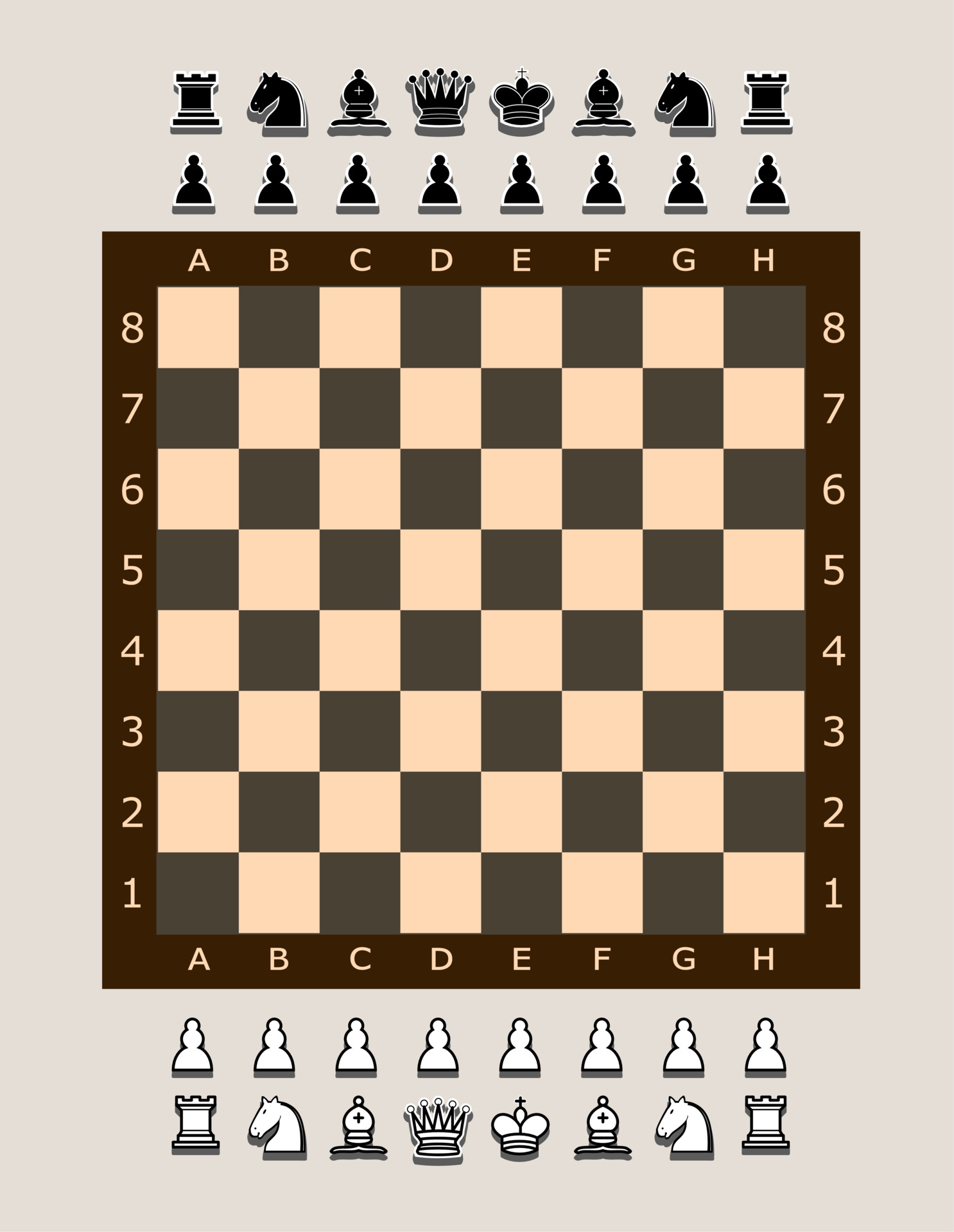
Let’s look at how chess works. First off, a chess board is a square shaped plane, divided into 64 smaller squares (Fig.1) . They are named using letters in the columns and numbers in the rows.
Now if we rest this board on its corners, the load of each piece from the board, this orientation is similar to a plate supported on four sides. Here the load from each piece will be distributed to the corners and the combined load from all the pieces will be transferred to the corner supports.
Now, in a game of chess, the pieces are usually static, i.e., they do not move. The only shift occurs when a player chooses to move a piece. This would occur by the player picking up their piece and placing it down in the new place on the board. While the player is picking up their piece, the weight of the piece being moved would be lost in the corners proportional to its position on the board and the sum of the weight lost at each corner would be equal to the weight of the piece being picked up. Similarly this is the same when we place the piece back, it will sense the change in weight and find its position again.
Location computation
Weight of the object ‘W’ is distributed among the four legs. The load cell readings placed produce the weights W1,W2,W3,W4 corresponding to each of the legs.
This problem can be reduced from a 3 dimensional problem into a 2 dimensional problem by decomposing it into two different parts to find the location of the point load along each axis of the surface. This resembles a simply supported beam.
The new weights of the legs L1 and L4 after converting into WL1’ and WL2’
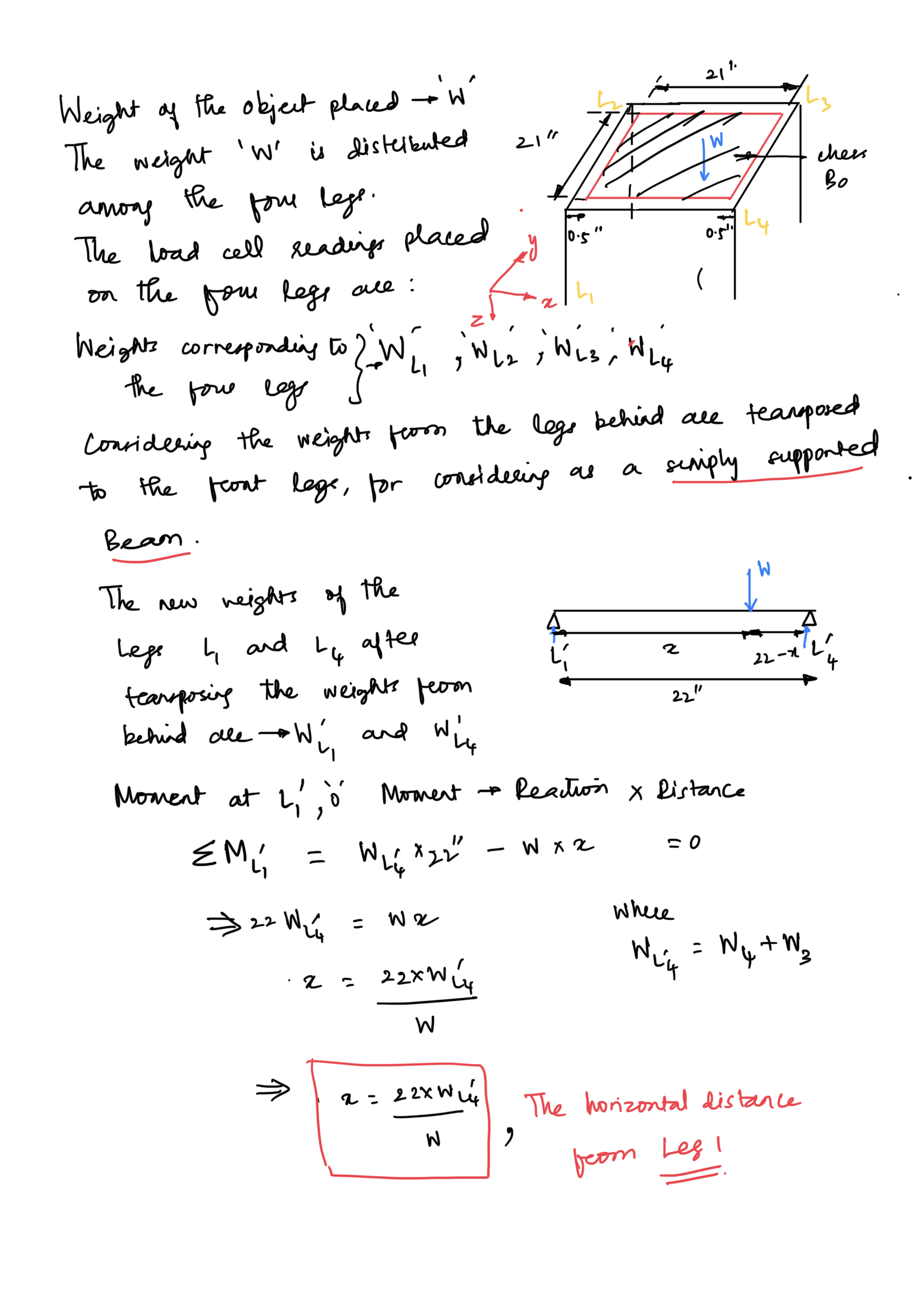
Using these equations (Fig 2), we can compute the location of the weight change occurred on the chess board. Based on the obtained x and y values we can classify the grid location as well.
Working of Sensors
The current measurement system contains the load cell as a primary sensing component. In the load cell, the strain experienced by the cell is directly proportional to the resistance (Fig 3). This change in resistance is translated into voltage. However, the voltage generated by the system is of a very low magnitude and this needs to be scaled appropriately. This amplification is done with the help of the HX711 amplifier. Broadly, the strain gauge works using the principle of Wheatstone bridge and these changes in resistance is translated to the voltage.
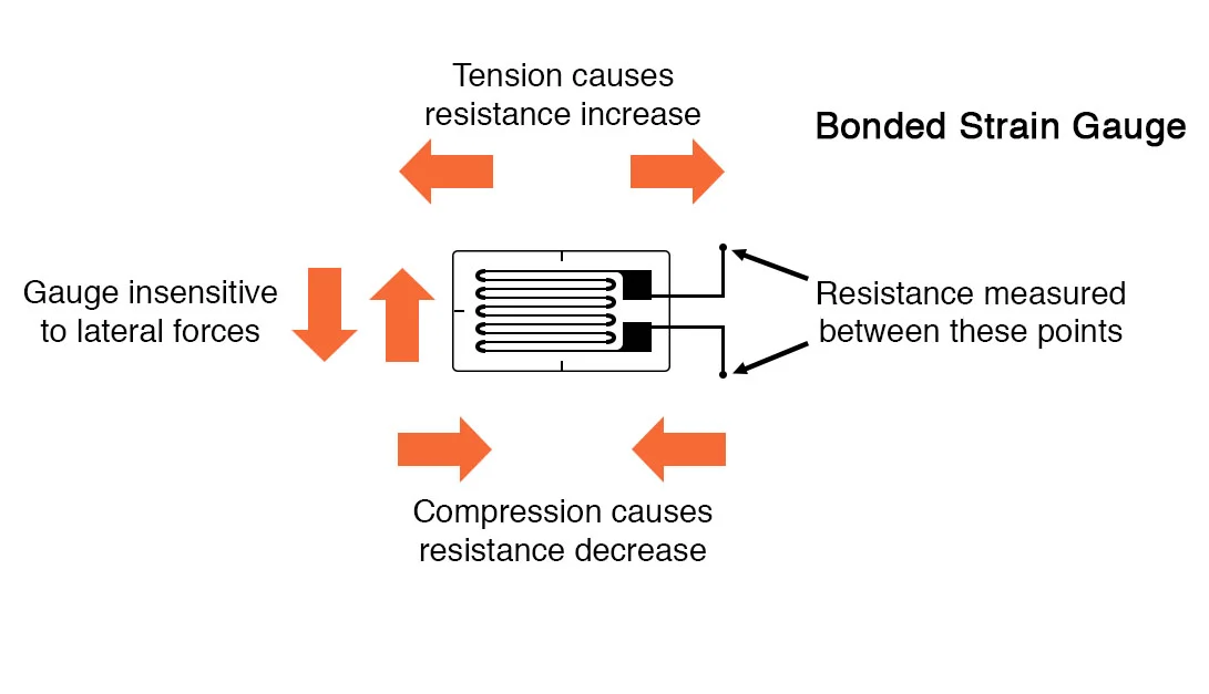
The design of the strain gauge is in consideration with the resistance of the strain gauge and the temperature. Firstly, we identify the resistance of the strain gauge and place resistors with same resistance in the circuit. When a voltage is applied to the Wheatstone bridge, a voltage difference is observed in the system which is proportional to the strain induced. But, when the strain induced is zero, the resulting voltage would be zero (as the bridge is balanced) and correspondingly, we can observe a change in voltage with respect to the exerted strain. In a nutshell, any small changes experienced by the strain gauge is recognized by the Wheatstone bridge and this creates a voltage difference.
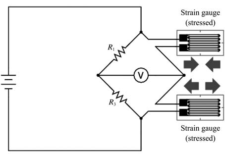
This way, the physical phenomenon of load, is translated into voltage. However, the consideration of strain gauge being temperature sensitive is a key factor as it inhibits getting appropriate readings. The sensitivity to change in temperature causes a change in voltage which in turn is misleading. To counteract this, a half-bridge circuit is preferred as(Fig 4). When two strain gauges are used, the change in resistance of each resistor is cancelled out which results in correct output. Also, it yields twice the output for a certain strain.
Mathematically, load cell can be defined as a second order system [4]:
Here, So denotes static gain, delta denotes damping and Omega which denotes resonance frequency.
Signal Conditioning
For the proper functioning of the load cell, it needs to be supplied with a regulated power source, a proper amplification mechanism, and an ADC conversion. Incorporating these three elements as separate entities in a circuit can increase the complexity both in terms of cost and time. To address these shortcomings, a breakout board such as HX711 can be used. For a better understanding, the current section eludes the working mechanism of the HX711 (Fig. 5 ).
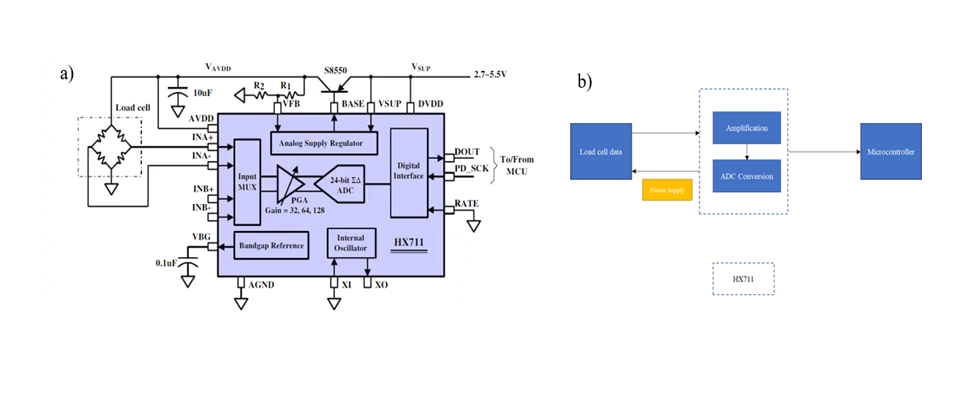
Initially, the amplifier provides the excitation voltage for the load cell to function and capture the readings. As the load cell captures the external changes, the analog data is then transmitted to the HX711 for converting into digital signals. The transmitted signal is passed through the Programmable Gain Amplifier via input multiplexer which can transmit , 128, 32 and 74 gain over A , B and A channels. Optimally, it is recommended to use 128 gain for better resolution of the signal. These generated analog signals require amplification as low strength signal might not be compatible with the rest of the Data Acquisition System.
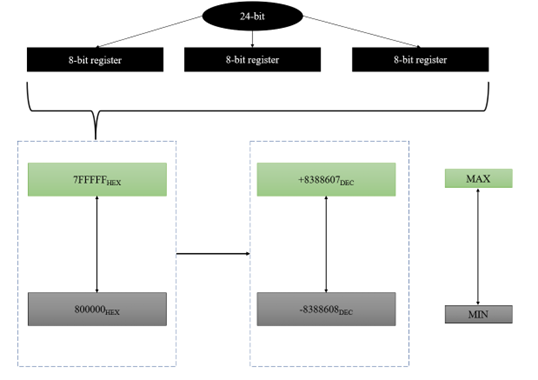
At a micro level, the ADC of the HX711 is connected to a common clock which samples at a rate of 80 SPS and the DOUT is connected to the microcontroller. Each time a pulse is send via the SCK , the ADC sends signal to the microcontroller via the DOUT pin. This data will be stored in the register with 8 bit each – 24 bit in total. Each pulse sent through SCK is responsible for data transfer via DOUT and storage in the register. After 24 pulses, all of the registries will be full and a final 25th pulse is sent to obtain the 128 gain (Fig.6) . The data stored in the registries in the Hexadecimal format within the range of 800000HEX and 7FFFFFHEX. The current hexadecimal range will be represented in a decimal format ( -8388608 to 8388607) which is further used by the microcontroller. These amplified digital signals are then further processed by the microcontroller to obtain a meaningful output.
The following table presents salient features and metrics of the HX711 [5] :
| Characteristic | Value |
|---|---|
| Pins | 16 |
| ADC bit | 24 |
| Output data coding | 2’s complement |
| Full scale differential input range V(inp) – V(inn) | ± 0.5 (AVDD/GAIN) |
| Operating supply voltage | 2.6 ~ 5.5V |
| Temperature range | -40 ~ +85 °C |
| Power supply | Normal operation <1.5mA Power down <1μA |
Table 1 : Salient metrics of HX711
Working of Instrument
Flowchart
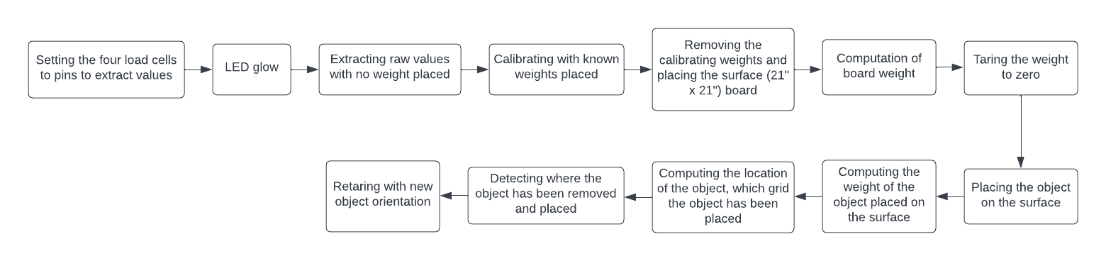
Initially, the experiment begins by extracting the pin values from each load cell using the existing HX711 package. The captured values are random and exhibit a certain level of noise. To counteract this, the sensor is left to capture the data, averaging for 10 times until the values stabilize. This is signaled to the user by the onboard LED on Pico. As a next step, the raw values are captured by the load cell using no weights and then using standard design weights. These values are stored as they would help in the initial calibration of system. Once the load cells are calibrated using the standard weights, a curve has been modeled for each of the load cell and this is utilized for further computation. As the final goal is to understand chess piece movement on a surface, the weight of the resting surface needs to be tared for quantifying the exact weight of each piece. Once the tare weight is obtained, the system is ready for weighing the magnitude of objects placed on the surface.
The next blocks elaborate on the rationale behind localization. The surface of the table has been divided into 2.68X2.68 grids to mimic the chess board configuration of 64 grids on a 21X21 inch board. Each grid is labeled similar to an actual chessboard in a A,B,C….. and 1,2,3,….. fashion. This will help in the per identification of the object in a grid to due to the well-defined boundary. The location of the object is identified each time, after getting the weight readings exceed a certain threshold, currently the threshold is 10 grams.
To minimize the computer interaction, a external button connected to the breadboard is utilized to advance from one block to another. Also, the onboard LED acts as a signal relaying the status of ongoing computation in Raspberry Pico.
Arrangement
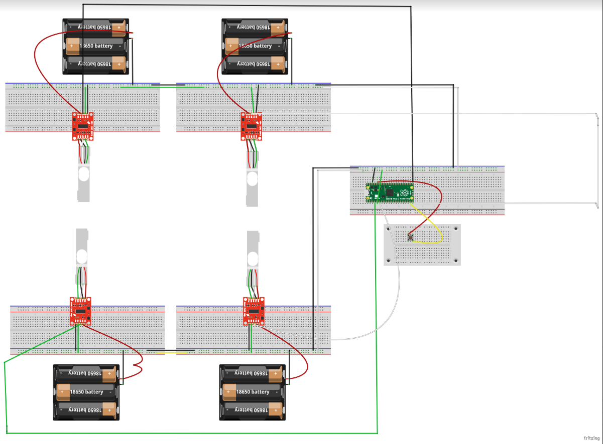
The approach for understanding the static loading is presented in the Figure 7. The study involves various electronic components such as sensors, microcontroller, amplifier, and buttons. Figure 8 presents the arrangement of the wires for the project. The board is placed on top of the four load cells. The SCK pins and the ground of the HX711 are all connected to a common respective terminal. The positive end of each power pack is connected to the VCC pin in the HX711 and the negative end was connected to the common ground terminal. A button is also connected to the Raspberry Pico W.
| Load cell | Data Pin | Clock Pin |
| 1 | 4 | 2 |
| 2 | 3 | 2 |
| 3 | 16 | 2 |
| 4 | 15 | 2 |
Table 2 : GPIO Connections of HX711 to Raspberry Pi Pico
Calibration of the Load Cells
Here the raw readings from the HX711 constantly vary each time the system is initiated. Hence a proper calibration is required for the load cells. We have used a linear fit along two different known weights in order to compute the slope and intercept of this line. Each load cell has a separate linear fit as the readings from all the load cells are noticeably different.
Initially, there will be no loads on the top of the load cells and this zero load condition will be used as the first point for the fit. This is done by using the average of 10 readings.
Once the readings are saved into a variable, a second known load is placed on the sensors and this is again stored. Using the known weights and the zero load condition we can find the equation of the linear fit as follows for each of the load cells.
where,
kwv = known weight value
kw = known weight
zwv = zero weight value
Position recognition
Now once the calibration process is complete, we can place the board and all the pieces on the top of the load cells. This board and chess piece weight is also saved and removed from the total load.
Now every time the weights are computed they will be at zero until a weight change occurs. This is tested with a threshold of 10 grams as the minimum weight of the chess pieces used for this setup was 11 grams.
When the combined load from all the load cells exceeds the threshold, the position of the load which was removed is computed with the formula,
Where,
W=total weight
and WL4 = transposed weights along L4
Where,
W=total weight
and WL3 = transposed weights along L3 and L2
Using these equations the coordinates are computed. The coordinates are divided using the floor operator in order to find the quotient. This quotient is used to identify which column or row the weight change has occurred. Once the position has been found, the weight is again tared with this new weight distribution to the legs.
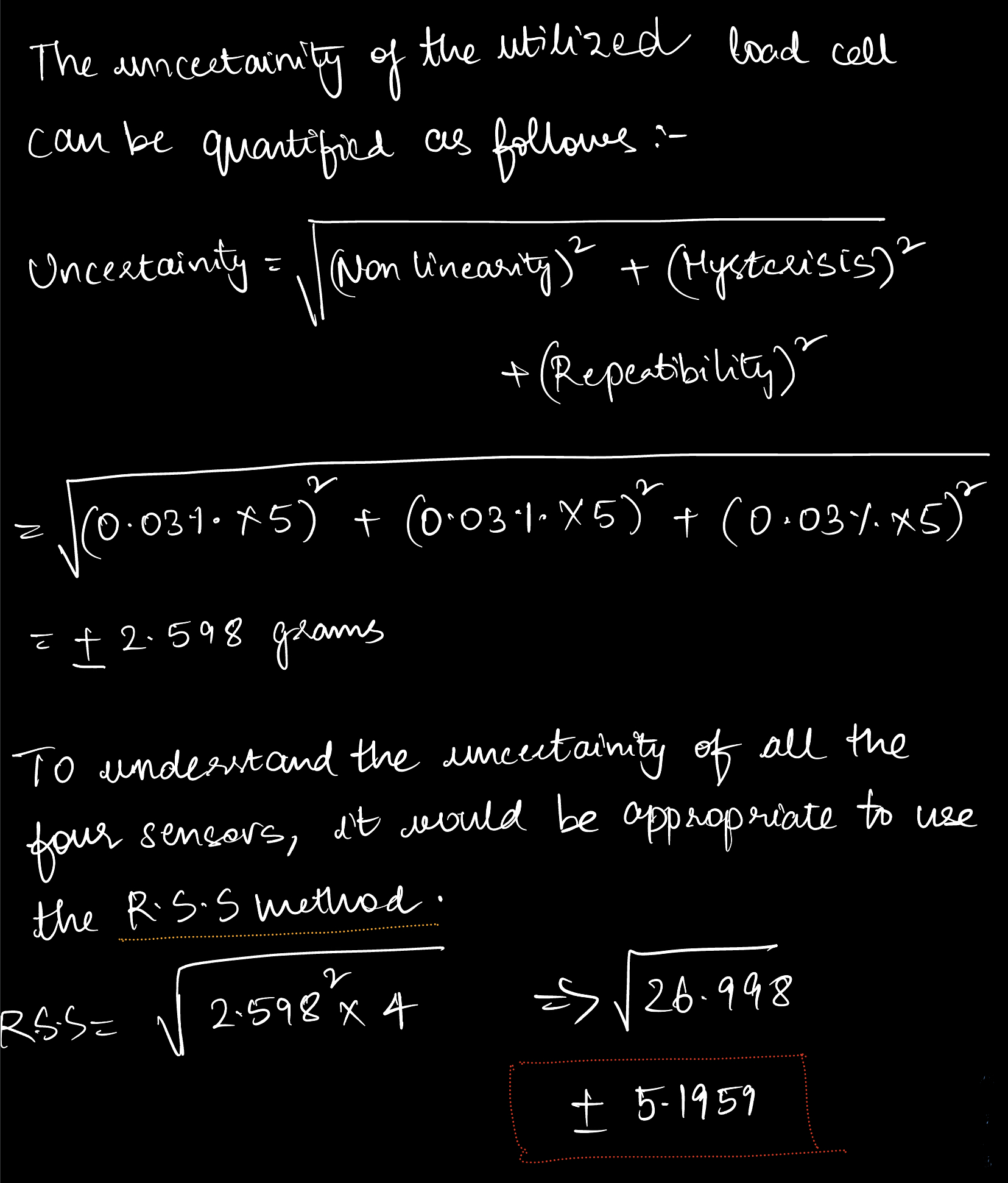
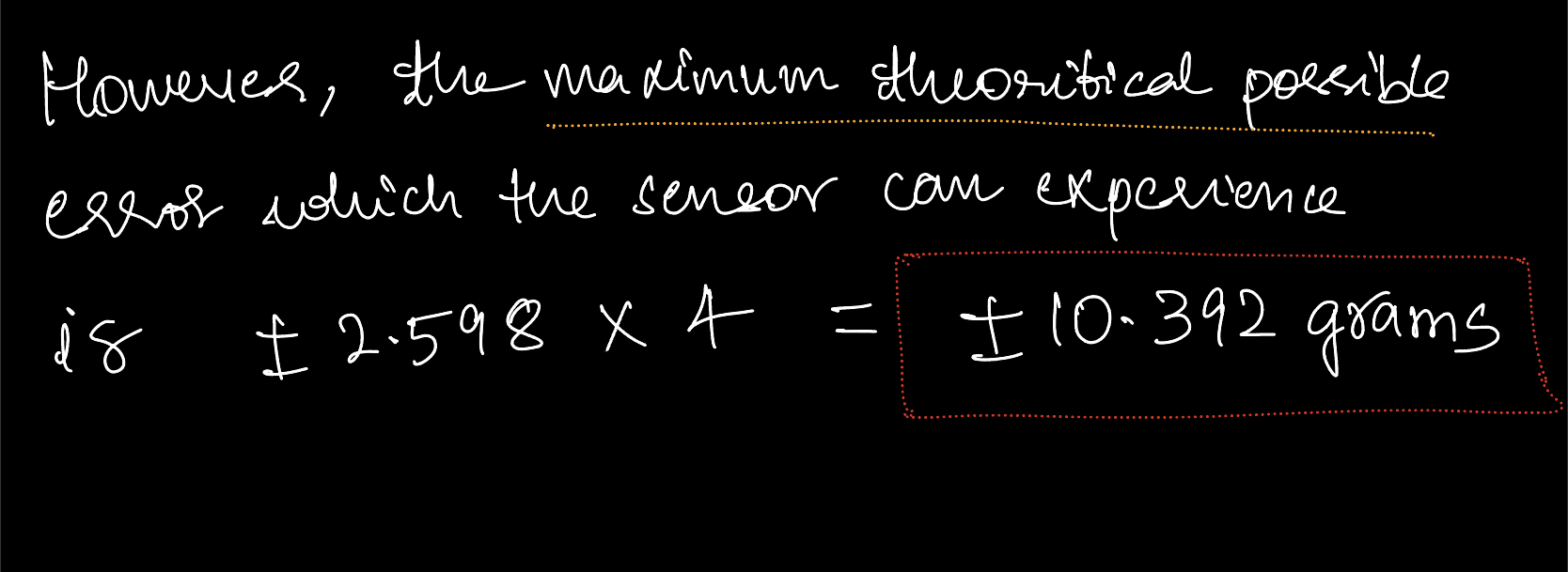
Uncertainty Estimation
Results
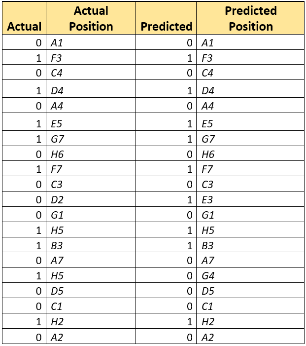
Based on a set of 20 observations (Fig 10), the accuracy of our sensing system has been identified as 90% (18/20). The table below depicts the actual and predicted position is given below
Code
The code for the project has been linked below. The modules used for the project are HX711[6], Machine, and Time.
Conclusion
The project aims to develop a system for identifying magnitude and localization of loads on a surface in a chess based setting. Here, we use four 5 kg load cells, coupled with HX711 amplifiers which are connected to the Raspberry Pico W. For calibrating the load cell, we used standard weights on each of the load cell to develop a linear fit. Further, calibrations for the custom designed table are performed. Load calculations are performed using existing HX711 package which result in the net load on the table. The surface is divided into 2.62 X 2.62 based grids to identify the location of the chess piece. The accuracy of the proposed system for localizing the load is found out to be 90% over 20 random experiments across different grids on the surface. As an extension, the system can be modified to identify multiple loading and dynamic changes on the surface.
We were successful to develop a real time load monitoring system to measure the weight of the object on the surface. We were able to find the position of the chess piece using the weight distribution of the object on the surface. The future steps for this project would be to keep a log of the moves of the pieces as well as integrate a web interface removing the need for connecting to a laptop in order to completely remove the dependency on a laptop.
Project update and progression
Project Proposal Presentation: 10/10/2022
Identified various papers and resources to select the best sensor which meet the project requirements.
Project Update: 10/18/2022
- Deployed a GitHub Page and decided on an appropriate load cell.
- Started to discuss the tentative flow of the code based on the sensors.
Project Update: 11/14/2022
Received the sensors from Prof. Bergés and started playing with them.
Project Update: 11/22/2022
Started with arrangement of the wires for the project and figured out that the connection to the Raspberry Pi Pico. We were also able to receive raw reading from the HX711 and started to change the code to calibrate it properly.
Project Update: 11/30/2022
Updated Prof Bergés about the calibration of the sensor and discussed about the data collection process for the project. Started to test the board putting chess pieces and board on the top. We came up with some solutions for the integration of the sensors.
Project Update: 12/05/2022
Completed the code to find out the position of the object placed on the board and updated Prof Bergés about the current status of the project. Prof Bergés suggested us to add button to remove the dependency on the computer. We wrote a new code to implement button on the project.
Logistics
The total list of items used
- Wooden frame -27 x 27 inch
- Square plate(chess board) - 22x22 inch
- Load cell (described below) x 4
- HX711 amplifier x 4
- Wires
- Batteries(AA) x 9
- Button - 1
- 3 battery holder x 4
- Known weights for calibration x4
- Weighing scale x1 (verifying the weights)
- Chess piece set x 1
Primarily, the logistics of the project can divided into two sections - electronic and non electronic hardware.
Non-electronic hardware:
For designing the table and fixing the sensors, the team has taken help from Brian Belowich. We initially consulted Brian for identifying the type of wood and the dimensions for the table. As the project progressed, we were in constant touch for additional hardware such as weighing scales, standard weights for calibration and nail connections.
Electronic hardware:
Initially, we visited TechSpark for soldering the amplifiers. Later, we continued to drop in for additional battery packs to obtain initial reading of the system. Also, we utilized the hardware tools for crimping the wires. This was essential in completing the circuit of the measurement system.
As the project progressed, we realized the need for longer connecting wires as the load cells were separated from the main microcontroller. But longer wires / jumper wires were not readily available in TechSpark. However, we salvaged longer wires from old transformers in the Autonomous Infrastructure Systems Lab by consulting Prof. Bergés.
Electronic Components
| Sensors | Serial / Make | Quantity | Purchase Link |
|---|---|---|---|
| Load Cell | 5Kg / 114990100 / Seeed Technology Co., Ltd | 4 | Amazon |
| Load Cell Amplifier | HX711 | 4 | SparkFun |
| Resistor Kit | 1/4W 500 pieces | 1 | CanaKit |

References
[1] https://www.vecteezy.com/vector-art/9932045-chess-board-and-pieces-vector
[2] All About Circuits, Ed., “Strain gauges: Electrical Instrumentation Signals: Electronics textbook,” Strain Gauges. [Online]. Available: https://www.allaboutcircuits.com/textbook/direct-current/chpt-9/strain-gauges/. [Accessed: 12-Dec-2022].
[3] Isavi, Salar & Mahmoudi, Asghar . Design, fabrication and evaluation of a mechanical transducer for real time measurement of tilth aggregate sizes. Agricultural Engineering International: CIGR Journal. 15. 130-137. (2013)
[4] S. Eichstädt, A. Link, and E. Clemens, “Dynamic Uncertainty for Compensated Second-Order Systems,” Sensors (Basel), vol. 10, no. 8, pp. 7621–7631, Aug. 2010.
[5] SparkFun, "24-Bit Analog-to-Digital Converter (ADC) for Weigh Scales,” [Online]. Available: https://cdn.sparkfun.com/datasheets/Sensors/ForceFlex/hx711_english.pdf [Accessed: 12-Dec-2022]
[6] Robert HH, HX711, (2022), GitHub repository